Processing Masks

Speed up Higher Level Processing using masks

This tutorial explains how to generate and use processing masks in the FORCE Higher Level Processing System.

Info

This tutorial uses FORCE v. 3.7.6

What are processing masks?

In the FORCE Higher Level Processing System, processing masks can be used to restrict processing and analysis to certain pixels of interest. The masks need to be in datacube format, i.e. they need to be raster images in the same grid as all the other data. The masks can - but don’t need to - be in the same directory as the other data. The masks should be binary images. The pixels that have a mask value of 0 will be skipped.

What is the advantage of using processing masks?

Processing masks speed up processing.
- For each processing unit (block within the tile), the analysis mask is read first. If no valid pixel is in there, all the other data are not input, and the block is skipped. As an example, when processing a country like Japan, and provide a land mask, you can speed up processing significantly as many blocks are skipped entirely.
- On the pixel level, invalid pixels are skipped, too. This is especially beneficial for CPU-heavy tasks, e.g. machine learning predictions. As an example, when computing a tree species classification, you can speed up processing substantially if you provide a forest masks.
Processing masks decrease data volume substantially.
- In the processed products, the pixels of no interest have a nodata value. As all FORCE output is compressed (unless you choose to output in ENVI format; I don’t recommend to do this), the compression kicks in nicely if you have used processing masks. You can easily decrease data volume by several factors.
Processing masks facilitate analyzing the processed data.
- In the processed products, the pixels of no interest have a nodata value. Thus, you don’t need to sort the pixels on your own, e.g. computing confusion matrices and classification accuracy is more straightforward to implement.

Generate processing masks

Option 1: from vector data to mask

FORCE comes with a program to generate processing masks from vector data (e.g. shapefile or geopackage):

force-cube -h

$ Usage: force-cube [-hvirsantobj] input-file(s)
$
$ optional:
$ -h = show this help
$ -v = show version
$ -i = show program's purpose
$ -r = resampling method
$       any GDAL resampling method for raster data, e.g. cubic (default)
$       is ignored for vector data
$ -s = pixel resolution of cubed data, defaults to 10
$ -a = optional attribute name for vector data. force-cube will burn these values
$       into the output raster. default: no attribute is used; a binary mask
$       with geometry presence (1) or absence (0) is generated
$ -l = layer name for vector data (default: basename of input, without extension)
$ -n = output nodate value (defaults to 255)
$ -t = output data type (defaults to Byte; see GDAL for datatypes;
$       but note that FORCE HLPS only understands Int16 and Byte types correctly)
$ -o = output directory: the directory where you want to store the cubes
$       defaults to current directory
$       'datacube-definition.prj' needs to exist in there
$ -b = basename of output file (without extension)
$       defaults to the basename of the input-file
$       cannot be used when multiple input files are given
$ -j = number of jobs, defaults to 'as many as possible'
$
$ mandatory:
$ input-file(s) = the file(s) you want to cube
$
$ -----
$    see https://force-eo.readthedocs.io/en/latest/components/auxilliary/cube.html

force-cube imports raster or vector data into the datacube format needed by FORCE. The output directory needs to contain a copy of the datacube definition (see The Datacube tutorial).

If used with vector data, the tool rasterizes the polygon vector geometries. By default, it burns the occurence of the geometry into a raster image, i.e. it assigns the value 1 to all cells that are covered by a geometry, 0 if not. The resulting masks are compressed GeoTiff images. Do not worry about data volume when converting from vector to raster data, because the compression rate is extremely high.

In the following example, we generate a processing mask for the administrative area of Vienna, Austria.

force-cube -o /data/europe/mask vienna.shp

$ 0...10...20...30...40...50...60...70...80...90...100 - done.
$ 0...10...20...30...40...50...60...70...80...90...100 - done.
$ 0...10...20...30...40...50...60...70...80...90...100 - done.
$ 0...10...20...30...40...50...60...70...80...90...100 - done.

In this example, Vienna is covered by four tiles, a cubed GeoTiff was generated in each tile:

ls /data/europe/mask/X*/vienna.tif

$ /data/europe/mask/X0077_Y0058/vienna.tif
$ /data/europe/mask/X0077_Y0059/vienna.tif
$ /data/europe/mask/X0078_Y0058/vienna.tif
$ /data/europe/mask/X0078_Y0059/vienna.tif

For speedy visuailzation, build overviews and pyramids:

force-pyramid /data/europe/mask/X*/*.tif
force-mosaic /data/europe/mask

$ computing pyramids for vienna.tif
$ 0...10...20...30...40...50...60...70...80...90...100 - done.
$ computing pyramids for vienna.tif
$ 0...10...20...30...40...50...60...70...80...90...100 - done.
$ computing pyramids for vienna.tif
$ 0...10...20...30...40...50...60...70...80...90...100 - done.
$ computing pyramids for vienna.tif
$ 0...10...20...30...40...50...60...70...80...90...100 - done.
$
$ mosaicking vienna.tif
$ 4 chips found.

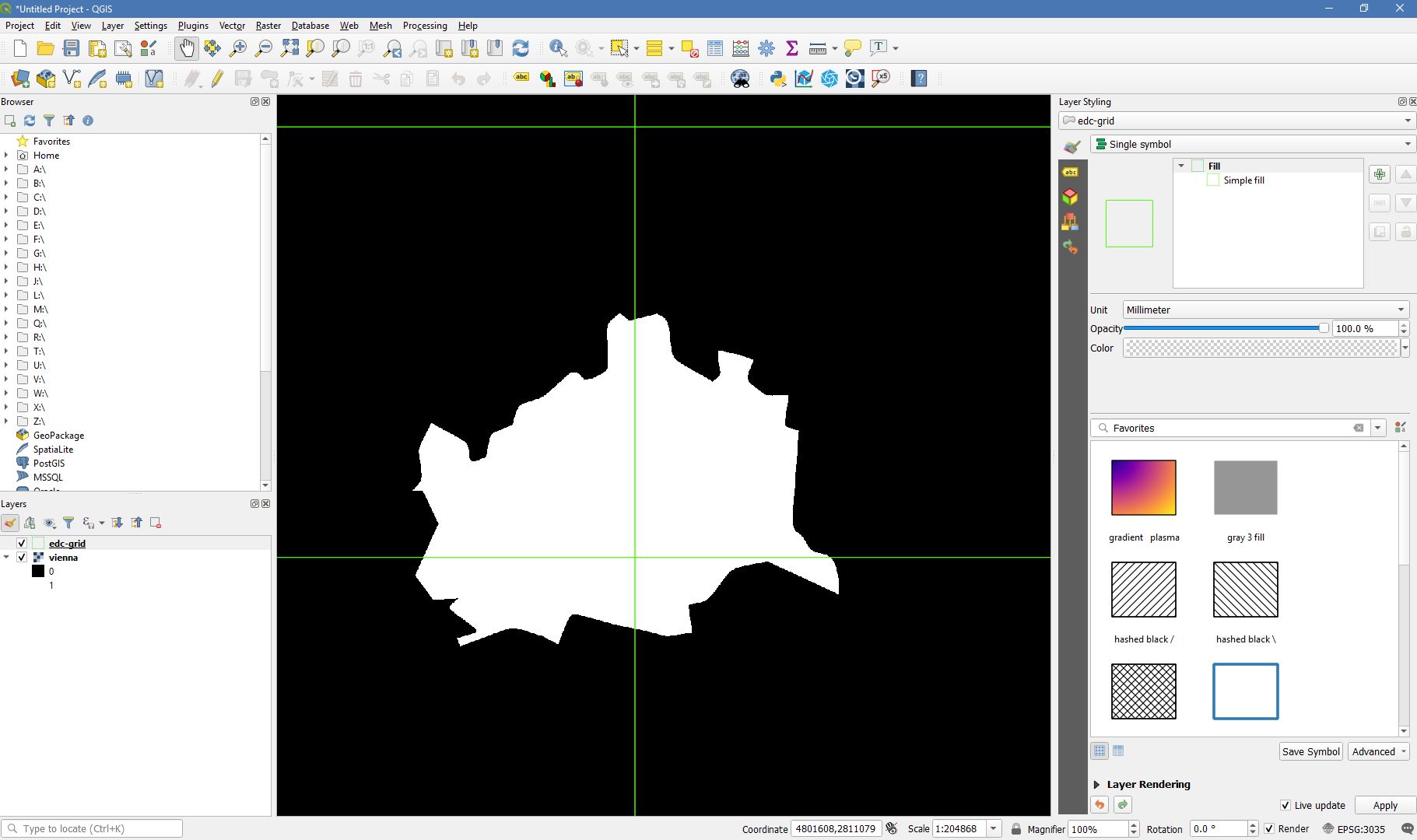
../_images/tutorial-mask-vector.jpg — *Mask of Vienna generated from a shapefile. Overlayed with the processing grid in green*

Option 2: from raster data to mask

FORCE comes with a program to generate processing masks from a raster image with continuous values:

force-procmask -h

$ Usage: force-procmask [-sldobj] input-basename calc-expr
$
$ optional:
$ -s = pixel resolution of cubed data, defaults to 10
$ -l = input-layer: band number in case of multi-band input rasters,
$       defaults to 1
$ -d = input directory: the datacube directory
$       defaults to current directory
$       'datacube-definition.prj' needs to exist in there
$ -o = output directory: the directory where you want to store the cubes
$       defaults to current directory
$ -b = basename of output file (without extension)
$       defaults to the basename of the input-file,
$       appended by '_procmask'
$ -j = number of jobs, defaults to 'as many as possible'
$
$ Positional arguments:
$ - input-basename: basename of input data
$ - calc-expr: Calculation in gdalnumeric syntax, e.g. 'A>2500'
$                The input variable is 'A'
$                For details about GDAL expressions, see
$                https://gdal.org/programs/gdal_calc.html
$
$ -----
$    see https://force-eo.readthedocs.io/en/latest/components/auxilliary/procmask.html

In the example given below, our input image is a multiband continuous fields dataset, which gives the percentages of built-up land (urban), high vegetation (trees), and low vegetation (grass, agriculture).

Note

If the data are not already in the datacube format, use force-cube to import the data (see the usage above). Use a raster resampling option to trigger the raster import, e.g. cubic (bc it’s all about cubes, eh?).

In our case, the data are already in datacube format, covering 597 tiles:

cd /data/europe/pred
ls X*/*.tif | head

$ X0052_Y0045/CONFIELD_MLP.tif
$ X0052_Y0046/CONFIELD_MLP.tif
$ X0052_Y0047/CONFIELD_MLP.tif
$ X0052_Y0048/CONFIELD_MLP.tif
$ X0052_Y0049/CONFIELD_MLP.tif
$ X0052_Y0050/CONFIELD_MLP.tif
$ X0052_Y0051/CONFIELD_MLP.tif
$ X0052_Y0052/CONFIELD_MLP.tif
$ X0052_Y0053/CONFIELD_MLP.tif
$ X0053_Y0045/CONFIELD_MLP.tif

We generate the masks using force-procmask, which internally uses gdal_calc.py for executing the raster algebra. Thus, the arithmetic expression must be given in gdalnumeric syntax, e.g. ‘A>3000’. A refers to our input image. If this is a multiband file, the desired band can be specified with the -l option (if not given, the first band is used). In our example input image, the tree percentage is in band 2 and the percentage values are scaled by 100 (i.e. 100% = 10000). To generate a mask with tree cover > 30%, we use the following:

cd /data/europe/pred

force-procmask \
   -o /data/europe/mask \
   -b forest-mask \
   -l 2 \
   CONFIELD_MLP.tif \
   'A>3000'


$ Computers / CPU cores / Max jobs to run
$ 1:local / 80 / 597
$
$ Computer:jobs running/jobs completed/%of started jobs/Average seconds to complete
$ ETA: 0s Left: 0 AVG: 0.00s  local:0/597/100%/0.1s

We now have one cubed mask for each input image in the mask directory:

ls /data/europe/mask/X*/forest-mask.tif | wc -l

$ 597

For speedy visuailzation, build overviews and pyramids:

force-pyramid /data/europe/mask/X*/forest-mask.tif
force-mosaic /data/europe/mask

$ computing pyramids for forest-mask.tif
$ 0...10...20...30...40...50...60...70...80...90...100 - done.
$ computing pyramids for forest-mask.tif
$ 0...10...20...30...40...50...60...70...80...90...100 - done.
$ computing pyramids for forest-mask.tif
$ 0...10...20...30...40...50...60...70...80...90...100 - done.
$ computing pyramids for forest-mask.tif
$ 0...10...20...30...40...50...60...70...80...90...100 - done.
$ ...
$
$ mosaicking forest-mask.tif
$ 597 chips found.

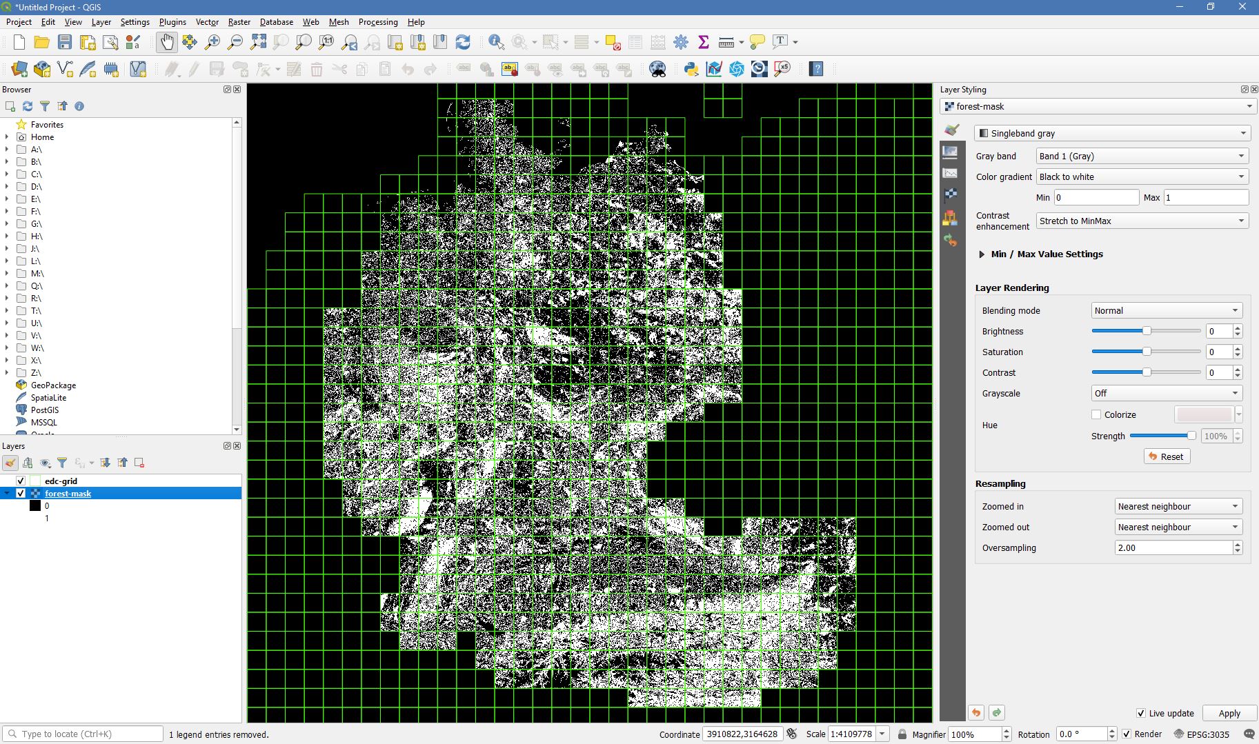
../_images/tutorial-mask-raster.jpg — *Forest mask generated from continuous raster input. Overlayed with the processing grid in green*

Use processing masks

Processing masks can easily be used in force-higher-level by setting the DIR_MASK and BASE_MASK parameters in the parameter file. They are the parent directory of the cubed masks, and the basename of the masks, respectively. To use the Vienna mask from above:

DIR_MASK = /data/europe/mask
BASE_MASK = vienna.tif

	This tutorial was written by David Frantz, main developer of FORCE, postdoc at EOL. Views are his own.





EO, ARD, Data Science, Open Science